Convolutional Neural Networks (CNN) are a state-of-the-art tool for Computer Vision tasks like image classification. They managed to improve performance for many image classification datasets in the past years. But what exactly are CNNs and how do they differ from conventional Neural Networks? In this article I will give you a high-level introduction in Convolutional Nets, their biological reference and how to build a CNN in Keras.
Overview
The structure of this article is as follows:
- Biological Reference
- Architecture Overview
- Layers
- Feature Extraction / Convolutional and Pooling Layers
- Classification / Fully Connected Layers
- A simple CNN for Image Classification in Keras
To proceed it is beneficial to have a basic understanding of Neural Networks but it is not required. I will try to write this post as if I was writing to my three-month-ago-me, which had no idea about CNNs. Anyway, I highly recommend reading this excellent lecture on Convolutional Nets by Andrej Karpathy at Stanford.
1. Biological Reference
I think it makes sense to include this part, as it explains where the ideas for Neural Networks come from. But I will try to make this short, since I am no neuroscientist. Most of what I write here, I know from this superb, informative article by Daphne Cornelisse (she IS a neuroscientist).
As babies we also had to learn to detect and label objects. Just like us an algorithm also has to see many (often millions) of pictures so that it is able to generalize and make predictions for pictures it hasn’t seen before.
Computers perceive images in a different way than us humans. Images are represented by 3-D arrays (\(height \times width \times depth\)). The height and width refer to those of the picture and the depth, the third dimension, refers to the three values necessary in the RGB color space to specify a color. For a computer, a picture therefore looks like 3D-Matrix like in the picture below.
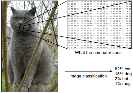
How computers see images, source: http://cs231n.github.io/
1.1 Neural Networks are inspired by biological neural systems
The origin of neural networks are the efforts to model the biological neural system. However, it since has become a topic of engineering and Machine Learning and with impressive results (for example at geolocating Google Street View images).
The artificial neuron is modelled based on the real biological neuron. The following picture shows the structure of a typical neuron. They consist mainly of three things, dendrites, soma (body), and axon.
 A biological (left) and mathematical (right) neuron model, source: http://cs231n.github.io/
Dendrites receive signals from surrounding neurons. Axons are a thin “tube” that transmit signals from neuron to other neurons. The contact from one axon to a dendrites is made with a synapse. The neuron then processes the received signals and outputs a signal (a.k.a “fire”) that has been modified or no signal at all. You can read more about biological neurons here.
Enough of biological neurons. The signals that travel along the axons are assumed to be \(x_0\) in the mathematical model, the “input” of the neuron. When the signal arrives on the synapse they interact. In Artificial Neural Networks this is modelled as the synapse having a set of weights. The signal is then multiplied the weights (\(x_0 \times w_0\)). The weights represent the influence other neurons have on the neuron at hand. If it is inhibitory weights are negative and if it is excitory the weights become positive. The idea of Neural Networks is that these weights are learnable. And what happens in the soma?
From the synapse the signal travels along the dendrites to the soma. There, all signals get summed up. Once a thertain threshold is reached within a limited time span the neuron fires. This firing is modelled with an activation function such as sigmoid \(\sigma(x) = 1/(1+ \exp^{-x})\) function. The activation function adds non-linearity to the Neural Network. This in important since many real-life contexts require non-linear thinking.
2 Architecture Overview
In normal NNs the neurons are normally modelled in layers of neurons, the so-called hidden layers. The most common layer type is the fully-connected layer where neurons of adjacent layers are connected (every pair of neurons has a connection). This is different in CNN architectures. Neurons in a layer only connect to a small region of the previous layer. This is represented in the following picture (the squares that are connected to smaller squares in the next layer). Additionally, for image classification tasks, there is one (or multiple) fully-connected layer(s) at the end to make the class predictions.
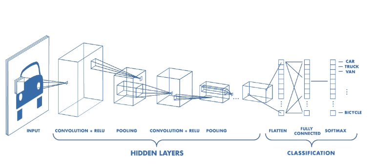
Architecture of a CNN. — Source: mathworks
3 Layers in a Convolutional Net
As mentioned above, the most common layers in Convolutional Neural Networks are Convolution, Pooling and Fully-Connected Layers. These layers are being stacked to form a ConvNet. A simple basic Architecture for ConvNet might look like this:
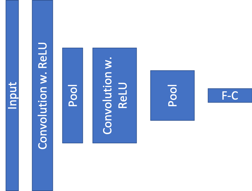 Simple CNN Architecture
Let’s get a quick overview what the layers do:
- Input Layer: The input layer is like the name says the input for the image. It takes a picture with a certain height and width and three R,G,B channels as depth.
- Convolution Layer: This layer calculates the feature space of the input. Every neuron is connected to an area of certain size in the previous layer (a.k.a receptive field). The output is calculated by taking the dotproduct between the input and the weights of the neuron.
- ReLU: The Rectified Linear Unit is the activation function
- Fully-Connected Layer: This layer computes the class scores. For example the MNIST dataset of digits contains 10 classes.
Let’s have a more detailed look at each of these layers/functions:
3.1 Convolutional Layer
You can imagine a Convolutional Layer as a filter moving across the whole picture doing a matrix multiplication at every position to produce an activation map. The idea of CNNs is that these filters will learn to activate when they receive a visual feature such as an edge, or a blotch of color. These high-level features are usually learned in the first layers of the network. The later layers will recognize shapes and finally objects as for example a head. The animation below shows how the 3x3 filter, also called kernel in some sources, slides over the input of size 5x5 to preduce an output of size 3x3. Have a look and try to understand what happens.
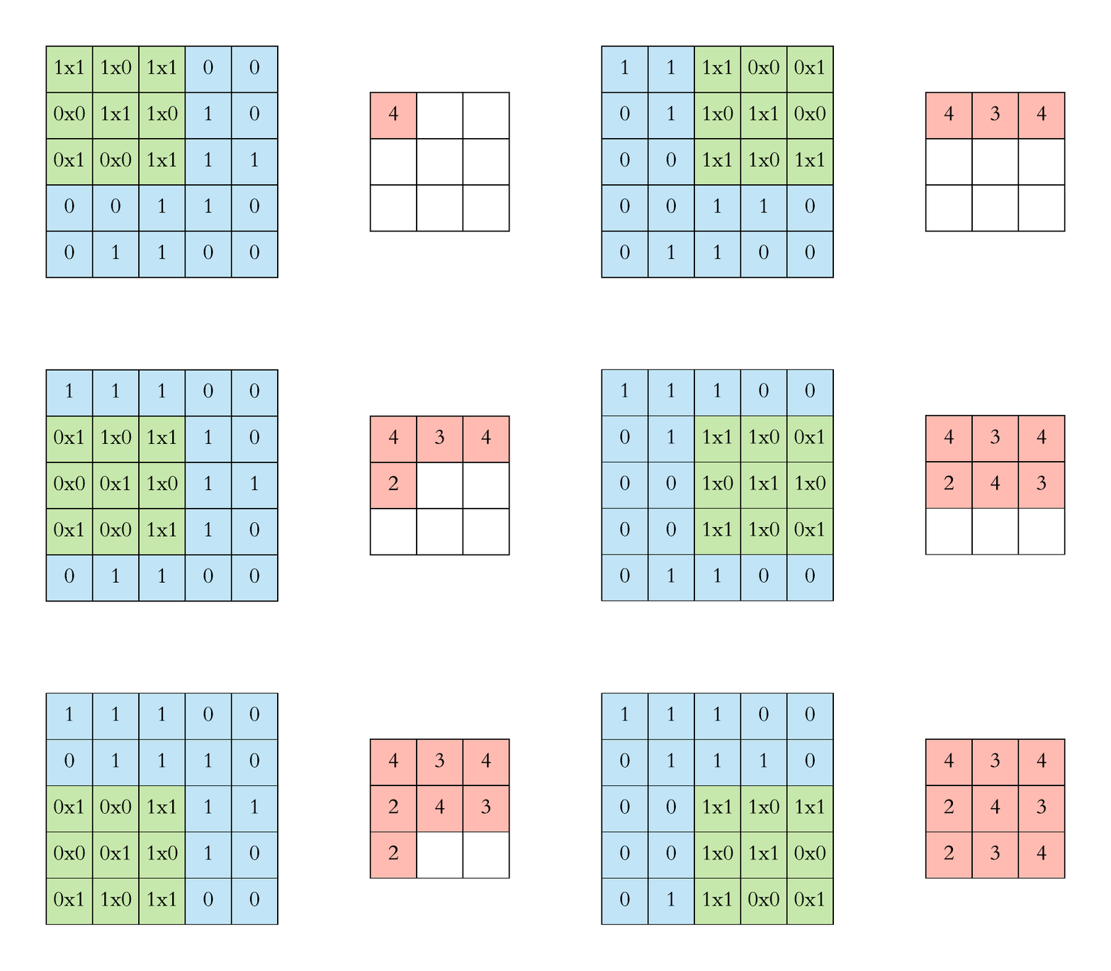 Filter sliding over input. Source: https://towardsdatascience.com/applied-deep-learning-part-4-convolutional-neural-networks-584bc134c1e2
As you can see, the filter contains a matrix of weights. In this simple 2D representation the calculation for one field (these fields are called receptive fields) is a simple dot product between the rows of the input and the columns of the weights. In a normal application the filter would also contain weights in the depth dimension.
Another aspect that you could notice is that, the output is of smaller size than the input. Often, this is not desired and the output is padded, i.e. the output gets fills up with zeros or the original values to keep the dimensions the same. The output would look like this then:
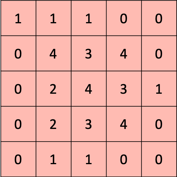
Padding of the output to keep input dimensions
Here I give you an overview of the hyperparameters that determine a Convolutional Layer:
| Hyperparamter | Values | Explanation |
|---|---|---|
| Filter size | Usually this would be (2x2; 3x3; 5x5) | This is the filter/kernel size that will move over the input. A bigger filter will produce a smaller output volume and generalize the data more. |
| Stride | Usually 1 or 2 | Determines how many pixels we move the filter each time it moves. A bigger stride will produce a smaller output volume. |
| Depth | It depends on the architecture you are using. Today’s very deep architectures can have up tp 512 filters. | The depth determine how many filters you want to convolve over your input. Each filter will look for something different in the input. |
| Zero-Padding | Depends on the output of the Convolutional Layer. Usually you want to keep the dimensions the same. Adjust your padding accordingly. (In Keras you just set the padding=”same” flag and it will do this automatically for you) | Adds values from the original input or zeros to the borders of the image so that the dimensions stay the same. |
There would be a lot more to write about Convolutional Layers but to keep the article within reasonable reading time I will leave it that. I will probably do a more detailed post on Convolutional Layers later. Feel free to ask me anything in the comments though.
3.2 ReLU Activation Function
The de-facto standard for activation functions at the moment is the ReLU function:
\(f(x)= \max(0,x)\)
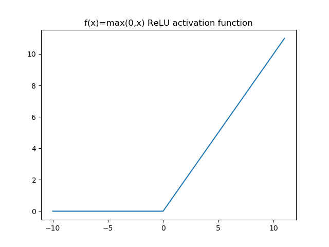
It is a fairly simple function that thresholds values at zero. The purpose is to introduce non-linearity into the network. ReLU functions have been shown to speed up the convergence of the stochastic gradient. To learn more about other activation functions and ReLU, check this out.
For the classification in the Fully-Connected Layer a different activation function will be used that is more suitable to the specific task (softmax function).
3.3 Pooling Layer
The pooling layer is a standard part of every CNN. It reduces the spatial size of the input and the number of parameters in the network. Like this it prevents overfitting on the training dataset and also diminishes computation. The most common Pooling Layer function is the MAX Pooling Layer. It also works with a filter of a certain size. The most common filter is of size 2x2 and a stride of 2. This sample Pooling Layer would halve the input height and width. The depth dimension stays constant as the pooling function is applied to every depth slice. For a visualization have a llok at the following figure:
 Pooling Layer with MAX function downsamples the input Source: CS231
3.4 Fully-Connected Layer
For image classification tasks the Fully-Connected Layer comes after the convolutions and pooling layers. Remember from the NN part that the neurons in these layers are connected to every layer of the previous layer?
There is only a dimensional problem. The output from the Conv + Pool layers are 3D and the FC Layer expects a 1D input. That is why a layer that “flattens” the 3D vector into a 1D vector is required. Don’t worry, this is also provided by Keras and you won’t have to do this manually. Finally, the FC layers (or multiple layers) computes the output for the classes.
Keras example
This standard Keras example shows a simple CNN for image classification on the MNIST dataset. The MNIST dataset is dataset of handwritten digits. The network then tries to classify the input into 10 available distinct digits. One of the advantages of the MNIST dataset is that you won’t need a GPU to train a CNN. So just go ahead copy+paste the code below and try undestand it at home. If you have any questions, recommendations please feel free to let me know in the comments or via e-mail.
With the fairly simple setup below I was able to get to an accuracy of 99.15%. Not bad, right?
from keras.layers import Conv2D, MaxPool2D, Flatten, Dense, Activation, Dropout
from keras.models import Sequential
from keras.optimizers import Adam
from keras.datasets import mnist
from keras.utils import to_categorical

(x_train, y_train), (x_test, y_test) = mnist.load_data()
img_rows, img_cols = 28, 28  # the input dimensions of the photos
num_classes = 10  # 10 distinct digits
epochs = 10  # number of epochs on dataset

x_train = x_train.reshape(x_train.shape[0], img_rows, img_cols, 1)
x_test = x_test.reshape(x_test.shape[0], img_rows, img_cols, 1)
input_shape = (img_rows, img_cols, 1)

x_train = x_train.astype('float32')
x_test = x_test.astype('float32')
# scaling down the images to [0 ,1]
x_train /= 255
x_test /= 255
print('x_train shape: {}'.format(x_train.shape))
print(x_train.shape[0], 'train samples')
print(x_test.shape[0], 'test samples')

# convert class vectors to binary class matrices also know as hot-one-encoding
y_train = to_categorical(y_train, num_classes)
y_test = to_categorical(y_test, num_classes)

model_clf = Sequential()

model_clf.add(Conv2D(filters=24, kernel_size=(2, 2), strides=(1, 1), padding='same', input_shape=input_shape))
model_clf.add(Activation('relu'))
model_clf.add(MaxPool2D(pool_size=(2, 2), strides=(2, 2)))
model_clf.add(Conv2D(filters=48, kernel_size=(2, 2), strides=(1, 1), padding='same'))
model_clf.add(Activation('relu'))
model_clf.add(MaxPool2D(pool_size=(2, 2), strides=(2, 2)))
model_clf.add(Flatten())
model_clf.add(Dense(512, activation='relu'))
model_clf.add(Dropout(0.5))
model_clf.add(Dense(128, activation='relu'))
model_clf.add(Dropout(0.5))
model_clf.add(Dense(10, activation='softmax')) # the final output vector will have shape (10,)

model_clf.compile(optimizer=Adam(), loss='categorical_crossentropy', metrics=['accuracy'])
model_clf.fit(x_train, y_train, batch_size=24, epochs=10, validation_data=(x_test, y_test))